Business Cycle Theory: The Economy in the Short Run презентация
Содержание
- 2. INTRODUCTION TO ECONOMIC FLUCTUATIONS INTRODUCTION TO ECONOMIC FLUCTUATIONS
- 3. 10-1 The Facts About the Business Cycle 10-1 The Facts About
- 4. 10-1 The Facts About the Business Cycle When the economy experiences
- 5. Real GDP Growth in the United States Growth in real GDP
- 6. Growth in Consumption and Investment Growth in Consumption and Investment
- 7. Unemployment The U rises significantly during periods of recession, shown
- 8. Okun’s Law This figure is a scatter plot of the
- 9. 10-1 The Facts About the Business Cycle What relationship should we
- 10. 10-1 The Facts About the Business Cycle GDP and Its Components
- 11. 10-1 The Facts About the Business Cycle Economists arrive at their
- 12. 10-1 The Facts About the Business Cycle Average WORKWEEK of production
- 13. 10-2 Time Horizons in Macroeconomics The theoretical separation of real and
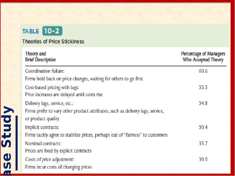
- 14. 2 If You Want to Know Why Firms Have Sticky Prices,
- 16. 10-2 Time Horizons in Macroeconomics How does the introduction of StP
- 17. 10-2 Time Horizons in Macroeconomics How the Short Run and Long
- 18. 10-3 Aggregate Demand Aggregate demand (AD) is the relationship between the
- 19. 10-3 Aggregate Demand The Quantity Equation as Aggregate Demand Why the
- 20. 10-3 Aggregate Demand The Quantity Equation as Aggregate Demand Why the
- 21. 10-3 Aggregate Demand We have assumed => M determines the
- 22. 10-3 Aggregate Demand The Quantity Equation as Aggregate Demand Why the
- 23. Shifts in the Aggregate Demand Curve Changes in the M shift
- 24. 10-4 Aggregate Supply The Long Run: The Vertical Aggregate Supply Curve
- 25. 10-4 Aggregate Supply The Long-Run Aggregate Supply Curve In the
- 26. 10-4 Aggregate Supply Shifts in Aggregate Demand in the Long Run
- 27. 10-4 Aggregate Supply The Short-Run Aggregate Supply Curve In this
- 28. 10-4 Aggregate Supply Shifts in Aggregate Demand in the Short Run
- 29. 10-4 Aggregate Supply Long-Run Equilibrium In the LR, the economy
- 30. 10-4 Aggregate Supply A Reduction in Aggregate Demand The economy
- 31. A Monetary Lesson From French History The story begins with the
- 32. David Hume on the Real Effects of Money Here is how
- 33. 10-5 Stabilization Policy Fluctuations in the economy as a whole
- 34. 10-5 Stabilization Policy An Increase in Aggregate Demand The
- 35. 10-5 Stabilization Policy Because supply shocks have a direct impact
- 36. 10-5 Stabilization Policy An Adverse Supply Shock An adverse
- 37. 10-5 Stabilization Policy Accommodating an Adverse Supply Shock In
- 38. How OPEC Helped Cause Stagflation in the 1970s and Euphoria in
- 39. 10-6 Conclusion This chapter introduced a framework to study economic fluctuations:
- 41. Скачать презентацию


 is the relationship between the")


Слайды и текст этой презентации
Слайд 1
Описание слайда:
Business Cycle Theory:
The Economy
in the Short Run
Слайд 2
Описание слайда:
INTRODUCTION TO ECONOMIC FLUCTUATIONS
INTRODUCTION TO ECONOMIC FLUCTUATIONS
Слайд 3
Описание слайда:
10-1 The Facts About the Business Cycle
10-1 The Facts About the Business Cycle
10-2 Time Horizons in Macroeconomics
10-3 Aggregate Demand
10-4 Aggregate Supply
10-5 Stabilization Policy
10-6 Conclusion
Слайд 4
Описание слайда:
10-1 The Facts About the Business Cycle
When the economy experiences a period of falling output and rising unemployment, the economy is said to be in recession.
U↑ , Y↓
Economists call these short-run fluctuations in output and employment the business cycle.
Before thinking about the theory of business cycles, let’s look at the facts that describe SRF in economic activity.
---------------------------
The official arbiter of when recessions begin and end is the National Bureau of Economic Research (NBER):
the stating date of each recession = the business cycle peak
the ending date = the business cycle trough.
Слайд 5
Описание слайда:
Real GDP Growth in the United States Growth in real GDP averages about 3% per year, but there are substantial fluctuations around this average.
Real GDP Growth in the United States Growth in real GDP averages about 3% per year, but there are substantial fluctuations around this average.
The shaded areas represent periods of recession.
Слайд 6
Описание слайда:
Growth in Consumption and Investment
Growth in Consumption and Investment
When the economy heads into a RECESSION, growth in
real consumption and
investment spending both decline.
Investment spending, shown in panel (b), is considerably more volatile than
consumption spending, shown in panel (a).
The shaded areas represent periods of recession
Слайд 7
Описание слайда:
Unemployment
The U rises significantly during periods of recession, shown here by the shaded areas.
Слайд 8
Описание слайда:
Okun’s Law
This figure is a scatter plot of the change in the UR on the horizontal axis and the % change in real GDP on the vertical axis, using data on the U.S economy.
Each point represents one year.
The figure shows that increases in U tend to be associated with lower-than-normal growth in real GDP. The correlation between these two variables is –0.89.
Слайд 9
Описание слайда:
10-1 The Facts About the Business Cycle
What relationship should we expect between U and real GDP?
Unemployed workers do not help to produce G&S =>
in↑ in the U rate should be associated with de↓ in real GDP.
This negative relationship between U and GDP is called Okun’s law.
Example:
The line drawn through the scatter of points tells us that
% Change in Real GDP= 3% − 2 x Change in U.
If the U remains the same, real GDP grows by about 3 % ;
If the U rises from 5 to 7%, then real GDP growth would be
% Change in Real GDP = 3% − 2 x (7% − 5%)= −1%.
Okun’s law says that GDP would fall by 1 % , indicating that the economy is in a recession.
Слайд 10
Описание слайда:
10-1 The Facts About the Business Cycle
GDP and Its Components
Unemployment and Okun’s Law
Leading Economic Indicators
Слайд 11
Описание слайда:
10-1 The Facts About the Business Cycle
Economists arrive at their forecasts is by looking at leading indicators,
which are variables that tend to fluctuate in advance of the overall economy.
Forecasts can differ in part because economists hold varying opinions about which leading indicators are most reliable.
The Conference Board announces the index of leading economic indicators.
This index includes ten data series
They are often used to forecast changes about 6-10 months into the future.
Слайд 12
Описание слайда:
10-1 The Facts About the Business Cycle
Average WORKWEEK of production workers in manufacturing.
A shorter workweek =>
lay off workers
cut back production
Average initial weekly claims for unemployment INSURANCE.
An in↑ in the number of new claims for U insurance =>
lay off workers
cutting back production
New orders for CONSUMER goods and materials, adjusted for inflation.↑↑
New orders for nondefense CAPITAL goods.↑↑
Index of supplier deliveries.
Slower deliveries indicate a future increase in economic activity.
New BUILDING permits issued↑↑
Index of STOCK prices. ↑↑
Money SUPPLY, adjusted for inflation. ↑↑
INTEREST rate spread.
A large spread =>
r are expected to rise,
economic activity increases.
Index of CONSUMER expectations. ↑↑
Слайд 13
Описание слайда:
10-2 Time Horizons in Macroeconomics
The theoretical separation of real and nominal variables is called the classical dichotomy.
The irrelevance of the M for the determination of real variables is called monetary neutrality.
Слайд 14
Описание слайда:
2 If You Want to Know Why Firms Have Sticky Prices, Ask Them
Слайд 15
Описание слайда:
Слайд 16
Описание слайда:
10-2 Time Horizons in Macroeconomics
How does the introduction of StP change our view of how the economy works? By S&D:
Слайд 17
Описание слайда:
10-2 Time Horizons in Macroeconomics
How the Short Run and Long Run Differ
The Model of Aggregate Supply and Aggregate Demand
Слайд 18
Описание слайда:
10-3 Aggregate Demand
Aggregate demand (AD) is the relationship between the quantity of Y demanded and the aggregate P.
The AD curve tells us the quantity of G&S people want to buy at any given P.
Here we use the quantity theory of money to provide a simple derivation of the AD curve.
---------------------------
From Ch.5
If V is constant => M determines the nominal value of Y,
nominal value of Y is the product of P & amount of Y.
The equation can be rewritten in terms of the S&D for real money balances (RMB):
Слайд 19
Описание слайда:
10-3 Aggregate Demand
The Quantity Equation as Aggregate Demand
Why the Aggregate Demand Curve Slopes Downward
Shifts in the Aggregate Demand Curve
Слайд 20
Описание слайда:
10-3 Aggregate Demand
The Quantity Equation as Aggregate Demand
Why the Aggregate Demand Curve Slopes Downward
Shifts in the Aggregate Demand Curve
Слайд 21
Описание слайда:
10-3 Aggregate Demand
We have assumed
=>
M determines the $ value of all transactions
Why the AD Curve Slopes Downward.
2 explanations:
If the P r↑, each transaction requires > $$, →
the # of transactions and =>
the quantity of G&S purchased
If Y is ↑er, people engage in > transactions and need ↑er M/P.
For a , ↑er M/P imply a ↓er P.
the ↑er level of M/P allows a > volume of transactions =>
> quantity of Y is demanded.
Слайд 22
Описание слайда:
10-3 Aggregate Demand
The Quantity Equation as Aggregate Demand
Why the Aggregate Demand Curve Slopes Downward
Shifts in the Aggregate Demand Curve
Слайд 23
Описание слайда:
Shifts in the Aggregate Demand Curve Changes in the M shift the AD curve.
In panel (a), a ↘ in the M reduces the nominal value of output PY.
For any given P, output Y is lower.
→ a ↘ in the M shifts the aggregate demand curve inward from AD1 to AD2.
In panel (b), an ↗ in the M raises the nominal value of output PY.
For any given P, output Y is higher.
→ an ↗in the M shifts the aggregate demand curve outward from AD1 to AD2.
Слайд 24
Описание слайда:
10-4 Aggregate Supply
The Long Run: The Vertical Aggregate Supply Curve
The Short Run: The Horizontal Aggregate Supply Curve
From the Short Run to the Long Run
Слайд 25
Описание слайда:
10-4 Aggregate Supply
The Long-Run Aggregate Supply Curve
In the lR, the level of output is determined by the amounts of K & L and by the T/L;
it does not depend on the price level.
The long-run aggregate supply curve, LRAS, is vertical.
Слайд 26
Описание слайда:
10-4 Aggregate Supply
Shifts in Aggregate Demand in the Long Run
A reduction in the M shifts the aggregate demand curve downward from AD1 to AD2.
The equilibrium for the economy moves from point A to point B.
Because the AS curve is vertical in the long run, the reduction in AD affects the P but not the level of output.
Слайд 27
Описание слайда:
10-4 Aggregate Supply
The Short-Run Aggregate Supply Curve
In this extreme example, all prices are fixed in the short run.
Therefore, the short-run aggregate supply curve, SRAS, is horizontal.
Слайд 28
Описание слайда:
10-4 Aggregate Supply
Shifts in Aggregate Demand in the Short Run
A reduction in the M shifts the AD curve downward from AD1 to AD2.
The equilibrium for the economy moves from point A to point B.
Because the AS curve is horizontal in the SR, the reduction in AD reduces the level of Y.
Слайд 29
Описание слайда:
10-4 Aggregate Supply
Long-Run Equilibrium
In the LR, the economy finds itself at the intersection of the LR AS curve and the AD curve.
Because prices have adjusted to this level, the SRAS curve crosses this point as well.
Слайд 30
Описание слайда:
10-4 Aggregate Supply
A Reduction in Aggregate Demand
The economy begins in long-run equilibrium at point A.
A reduction in AD, perhaps caused by a decrease in the M ,
moves the economy from point A to point B, where output is below its natural level.
As prices fall, the economy gradually recovers from the recession, moving from point B to point C.
Слайд 31
Описание слайда:
A Monetary Lesson From French History
The story begins with the unusual nature of French money at the time. The
money stock in this economy included a variety of gold and silver coins that, in
contrast to modern money, did not indicate a specific monetary value. Instead, the
monetary value of each coin was set by government decree, and the government
could easily change the monetary value and thus the M . Sometimes
this would occur literally overnight. It is almost as if, while you were sleeping,
every $1 bill in your wallet was replaced by a bill worth only 80 cents.
Indeed, that is what happened on September 22, 1724. Every person in France
woke up with 20 % less money than he or she had the night before. Over
the course of seven months, the nominal value of the money stock was reduced
by about 45 % . The goal of these changes was to reduce prices in the
economy to what the government considered an appropriate level.
Слайд 32
Описание слайда:
David Hume on the Real Effects of Money
Here
is how Hume described a monetary injection in
his 1752 essay Of Money:
To account, then, for this phenomenon, we must
consider, that though the high price of commodities
be a necessary consequence of the increase of gold
and silver, yet it follows not immediately upon that
increase; but some time is required before the money
circulates through the whole state, and makes its
effect be felt on all ranks of people. At first, no
alteration is perceived; by degrees the price rises, first
of one commodity, then of another; till the whole at
last reaches a just proportion with the new quantity
of specie which is in the kingdom. In my opinion,
it is only in this interval or intermediate situation,
between the acquisition of money and rise of prices,
that the increasing quantity of gold and silver is
favorable to industry.
Слайд 33
Описание слайда:
10-5 Stabilization Policy
Fluctuations in the economy as a whole come from changes AS or AD.
Economists call exogenous events that shift these curves shocks to the economy.
a shock that shifts the AD curve is called a demand shock.
a shock that shifts the AS curve is called a supply shock.
These shocks disrupt the economy by pushing output and employment away from their natural levels.
Goals of the model of AS & AD:
to show how shocks cause economic fluctuations.
to evaluate how macroeconomic policy can respond.
The stabilization policy is a policy aimed to reduce the severity of SR economic fluctuations.
Слайд 34
Описание слайда:
10-5 Stabilization Policy
An Increase in Aggregate Demand
The economy begins in long-run equilibrium at point A.
An increase in AD, perhaps due to an increase in the velocity of money, moves the economy from point A to point B, where Y is above its natural level.
As prices rise, output gradually returns to its natural level, and the economy moves from point B to point C.
Слайд 35
Описание слайда:
10-5 Stabilization Policy
Because supply shocks have a direct impact on the price level, they are sometimes called price shocks.
Examples:
■ A drought that destroys crops.
The reduction in food supply pushes up food P.
■ A new environmental protection law that requires firms to reduce their emissions of pollutants.
Firms in↗ P.
■ An increase in union aggressiveness.
This pushes up wages and the prices.
■ The organization of an international oil cartel.
By curtailing competition, the major oil producers can raise the world P of oil.
All these events are adverse supply shocks, which means they push costs and prices upward.
A favorable supply shock reduces costs and prices.
Слайд 36
Описание слайда:
10-5 Stabilization Policy
An Adverse Supply Shock
An adverse supply shock pushes up costs and thus prices.
If AD is held constant, the economy moves from point A to point B, leading to stagflation - a combination of increasing prices and falling output.
Eventually, as prices fall, the economy returns to the natural level of Y, point A.
Слайд 37
Описание слайда:
10-5 Stabilization Policy
Accommodating an Adverse Supply Shock
In response to an adverse supply shock,
the Fed can increase AD to prevent a reduction in output. The economy moves from point A to point C.
The cost of this policy is a permanently higher level of prices.
Слайд 38
Описание слайда:
How OPEC Helped Cause Stagflation in the 1970s and Euphoria in the 1980s
Слайд 39
Описание слайда:
10-6 Conclusion
This chapter introduced a framework to study economic fluctuations:
the model of aggregate supply and aggregate demand.
The model is built on the assumption that prices are sticky in the short run and flexible in the long run.
It shows how shocks to the economy cause output to deviate temporarily from the level implied by the classical model.
The model also highlights the role of monetary policy.
On the one hand, poor monetary policy can be a source of destabilizing shocks to the economy.
On the other hand, a well-run monetary policy can respond to shocks and stabilize the economy.
Слайд 40
Описание слайда:
Скачать презентацию на тему Business Cycle Theory: The Economy in the Short Run можно ниже: